Seating 10 people at a dinner table has 3.6 million combinations.
If your business is leaving 10% on the table, you aren’t just losing efficiency, you’re missing the kind of gains that translate directly into millions in profit. You are in the right place to fix that.
If your business needs are to find the absolute best combination, whether it’s the most profitable schedule for your workforce, the perfect route for your delivery fleet, or the ideal stock levels for your warehouse, then you are not looking for ‘Generative AI‘ you are looking for Optimization.
Scheduling 50 nurses for a month has more combinations than atoms in the universe.
To understand why we need specialized AI algorithms, we first need to visualize the “Search Space.”
This is simply the total number of possible ways you could solve a problem. If you are using a spreadsheet or a human scheduler for this, you aren’t “optimizing.” You are essentially walking into a library the size of the galaxy, picking the first book you see, and saying, “This is the best book in the library.”
An optimization algorithm is essentially a high-speed, intelligent navigator for a landscape of billions of possibilities. Instead of checking every single option one by one, which would take centuries, it uses a mathematical score of quality to guide its search. It starts with a few random guesses, evaluates how good they are, and then iteratively improves them by keeping the best traits and discarding the failures.
It continues this process of “evolution” or “gradient descent” until it converges on the single best solution that maximizes your goal (like profit) while strictly obeying your constraints (like budget or time).
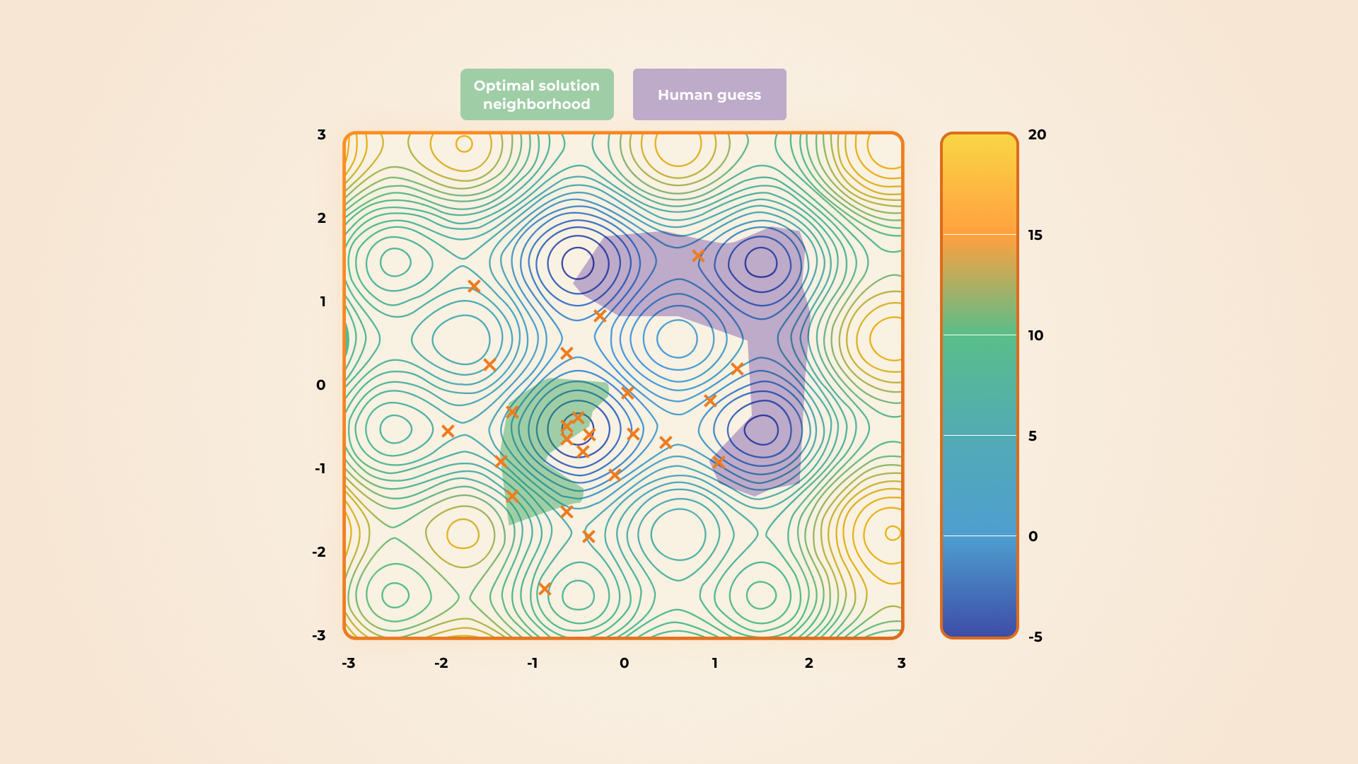
In a search space this massive, the difference between a “human guess” (a random point in the space) and the “mathematical optimum” (the highest peak) is usually 15% to 30%.
Imagine a mid-sized logistics company with 500 delivery trucks.
- Annual Operating Cost: $50,000 per truck (fuel, maintenance, driver wages).
- Total Spend: $25 Million / year.
The “Human Guess” (Current State):
Dispatchers manually assign routes based on zip codes. It works, but routes overlap, and trucks often drive empty or backtrack. They achieve 85% efficiency.
The “Mathematical Optimum” (Optimization Algorithm):
An algorithm processes millions of route combinations overnight. It finds a sequence that reduces total mileage by just 20% (a conservative optimization gain).
The Financial Reality:
20% Efficiency Gain = $5 Million saved in pure bottom-line profit.
That is the cost of “Good Enough.” You are currently spending $5 Million every year just because you cannot see the optimal route in the massive search space. The algorithm costs a fraction of that to run.
The Right Tool for the Job: Why LLMs Can’t Optimize (But Can Architect)
When you ask LLMs to “optimize a delivery schedule,” it doesn’t actually simulate trucks driving on a map. It doesn’t calculate fuel costs or driver fatigue. It simply asks itself: “Statistically, what word comes next in a sentence about delivery schedules?“
LLMs predict the next word. They cannot “backtrack” or “explore” billions of options to check if a specific route is valid.
They just guess. If the guess is wrong (e.g., assigning a truck to two places at once), the model doesn’t know until it’s too late.
In contrast, Optimization Algorithms are designed specifically to “evolve” answers over time.
They don’t guess; they test. They generate a thousand potential schedules, mathematically score them against your constraints, keep the top 10% that work, and discard the failures. They repeat this process for thousands of generations until they converge on a mathematically proven peak.
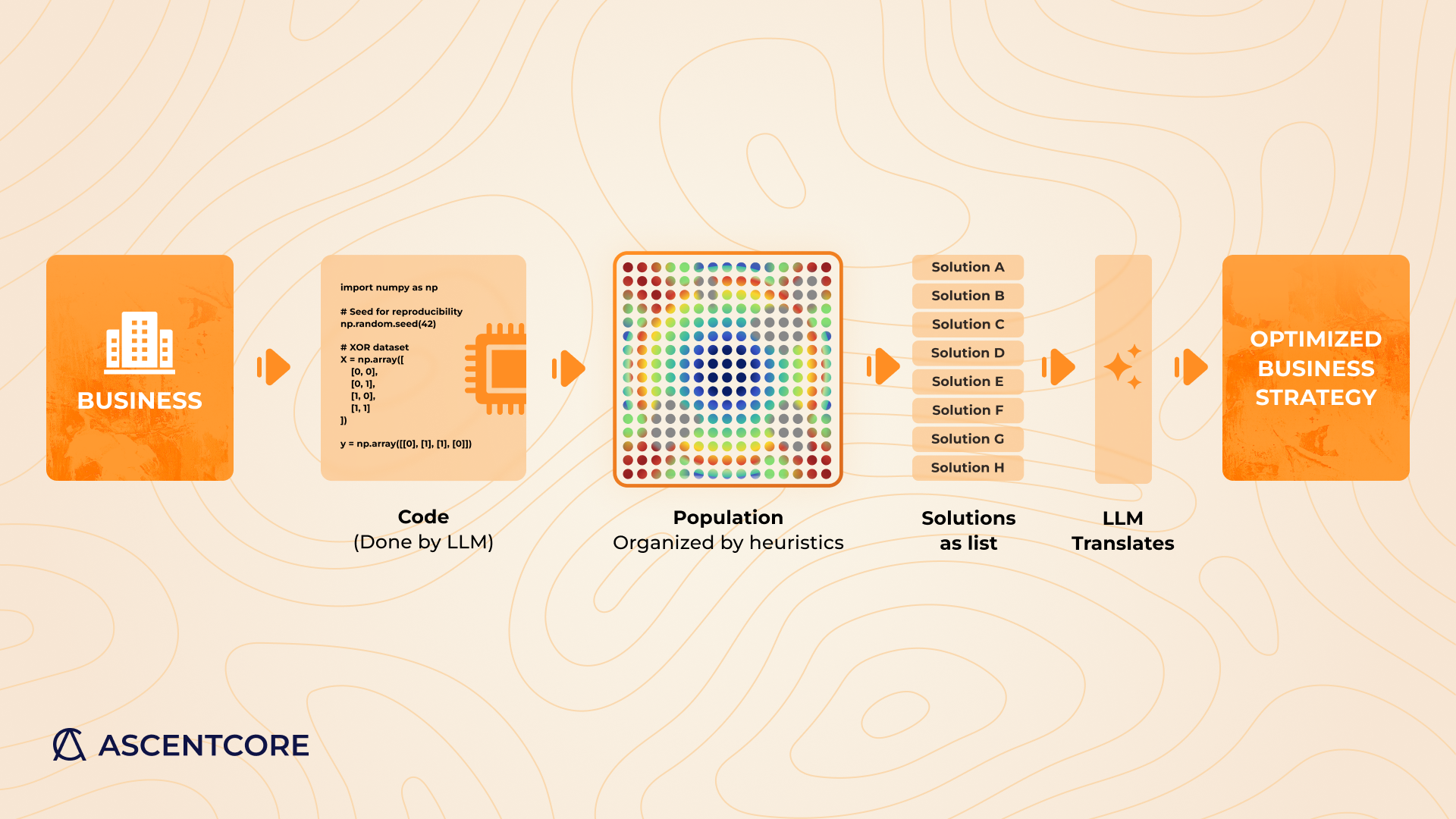
If algorithms are so powerful, why isn’t everyone using them? Because they speak Math, and businesses speak English.
While LLMs are terrible at searching the solution space, they are phenomenal at translating intent. They can bridge the gap between a CEO’s vision and an algorithm’s requirements.
Writing a mathematical model for a complex business problem, defining the Objective Function, the Hard Constraints (cannot happen), and the Soft Constraints (should be avoided) is incredibly difficult. It usually requires a PhD in Operations Research and weeks of coding, and this is where the LLM shines.
The Business Input:
“We need to maximize profit, but we can’t overwork our mechanics, and we never want to run out of brake pads.”
The Iterative Loop: Refining the Constraints
Optimization is rarely a “one-shot” process. Often, the first “optimal” solution reveals constraints you forgot to mention.
Example:
- Run 1: The algorithm returns a schedule that maximizes profit by having your top mechanic work 18 hours straight.
- The Realization: You realize, “Oh wait, that’s illegal. We have a union rule about 8-hour shifts.”
- The Refinement: You tell the LLM, “Add a constraint that no shift can exceed 8 hours.”
- Run 2: The LLM updates the mathematical model, the algorithm runs again, and produces a new solution that respects the law and maximizes profit within that new boundary.
This creates a powerful feedback loop. The LLM empowers business experts, the people who truly understand the nuances of the company to interact directly with high-end mathematics.
You describe the problem. The LLM architects the math. The Algorithm solves the puzzle. The LLM translates the solution back to you. You refine the problem.
This cycle turns optimization from a black-box engineering task into a dynamic business conversation. The result is a solution that is not just mathematically “perfect,” but practically applicable to your specific reality.
The hidden profit the human guess approach is missing
Here is how we uncovered the hidden millions your current process simply cannot see. To move from theory to evidence, we executed this “Business-to-Math” architecture across a series of complex, real-world benchmarks. We tested the system’s ability to interpret vague human constraints and convert them into rigorous evolutionary algorithms in three distinct domains:
- High-Volume Inventory,
- Streaming Content Scheduling,
- Asset ROI Maximization.
The following chapters detail these experiments, showcasing the actual code generated, the constraints discovered, and the optimized results that prove why translation, not generation, is the true power of LLMs in operations.
Use Case 1: Perishable Inventory Routing
The Scenario: Apex Heritage Orchards manages a high-volatility portfolio of perishable assets (7 apple and 4 pear varieties). The business faces a “race against entropy”: fruit quality degrades hourly while market windows close rapidly.
The goal is to maximize revenue by routing specific batches to one of seven distinct market tiers ranging from “Ultra-Premium” chefs to “Juice Press” salvage outlets before their biological value reaches zero.
The Business Friction: Traditional First-In-First-Out (FIFO) logistics fail here due to extreme variance in two areas:
- 1. Biological Variance: The portfolio ranges from the fragile Honeycrisp (Decay Rate: 2.5) to the highly durable Blue Delicious (Decay Rate: 0.3). A delay that is negligible for a Blue Delicious is catastrophic for a Honeycrisp.
- 2. Market Inflexibility: High-value markets have unforgiving windows. The “Ultra-Premium” market offers a 3.0x payout but rejects produce older than 2 days. The “Juice Press” accepts produce up to 60 days old but pays only 0.1x.
The “Human Guess” Approach: Warehouse managers typically rely on visual cues like “FIFO” or “Cherry Picking.” They see a pristine Honeycrisp and immediately rush it to the Ultra-Premium Chef for a 3x payout. They ignore that its aggressive 2.5 decay rate will mathematically drop its quality to 95.5 during transit just missing the strict 96.0 cutoff. By chasing this “home run,” they trigger a total rejection and a 90% revenue loss, while simultaneously clogging the loading dock with durable Blue Delicious apples that could have waited.
The Optimization Outcome: The engine calculated the theoretical value of every crate against decay curves, assigning channels based on “Value Retention Potential.”
- Honeycrisp (Decay 2.5): Routed to Local Fresh Market (M2). Analysis: Strategic Downgrade. Misses Ultra-Premium (96) by 0.5 points. Correctly routed to M2 (>85) to avoid total loss.
- Bartlett Pear (Decay 3.0): Routed to Local Fresh Market (M2). Analysis: Critical Precision. Arrives on Day 2 with score 86.0 (Threshold 85). Any delay would force a downgrade.
- Blue Delicious (Decay 0.3): Routed to Regional Supermarket (M6). Analysis: Perfect Fit. Low initial quality (75) makes it ineligible for higher tiers, but M6 lists it as a “Preferred Product.”
The Strategic Insight: The “Blue Delicious Factor” revealed that holding durable inventory (like Blue Delicious) allows for “Distressed Product” windows later, freeing up immediate processing capacity for high-maintenance varieties like Bartlett Pears.
| Product | Assigned Market | Delivery Day | Decay Rate | Calculated Quality | Strategic Analysis & Source Validation |
| Apple Honeycrisp | Local Fresh Market (Matches M2) | Day 1 | 2.5 | 95.5 | Strategic Downgrade. Misses M1 Ultra-Premium cutoff (96) by 0.5 points. Correctly routed to M2 (Req: >85) to avoid rejection. |
| Pear Bartlett | Local Fresh Market (Matches M2) | Day 2 | 3.0 | 86.0 | Critical Precision. Arrives just 1 point above the M2 rejection threshold (85). Any delay would force a downgrade to M4/M5. |
| Apple PinkLady | Local Fresh Market (Matches M2) | Day 1 | 1.5 | 93.5 | Optimal. M2 lists Pink Lady as a “Preferred Product,” ensuring volume acceptance. |
| Apple Fuji | Local Fresh Market (Matches M2) | Day 1 | 1.2 | 86.8 | Secured. safely clears the M2 quality floor (85). |
| Apple GrannySmith | Local Fresh Market (Matches M2) | Day 1 | 0.8 | 89.2 | Liquidity Focus. High durability (0.8 decay) would allow longer storage, but immediate sale clears inventory. M3 prefers this, but requires >70 quality and limits age to 10 days. |
| Pear Bosc | Regional Supermarket (Matches M6) | Day 2 | 1.8 | 84.4 | Volume Play. Bosc is preferred by M3 (Niche), but M6 (Discounter) ensures sales for lower quality scores. |
| Pear Anjou | Export Market B | Day 2 | 1.1 | 82.8 | Market Gap. Score is too low for M2 (>85) but fits M4 (Performance, >80) or M5 (Safety Net, >60). |
| Apple RedDelicious | Regional Supermarket (Matches M6) | Day 1 | 0.3 | 74.7 | Perfect Fit. M6 (High Volume) specifically lists Red Delicious as a “Preferred Product”. Low initial quality (75) makes it ineligible for higher tiers. |
| Apple Gala | Export Market B | Day 1 | N/A* | N/A | Note: M6 lists Gala as a “Preferred Product”, suggesting this export route might be an M6 equivalent. |
| Pear Comice | Local Fresh Market | Day 2 | N/A* | N/A | Note: Variety not listed in Source technical specs. Assumed to meet M2 threshold (>85). |
| Pear_Forelle | Local Fresh Market | Day 2 | N/A* | N/A | Note: Variety not listed in Source technical specs. Assumed to meet M2 threshold (>85). |
Use Case 2: Ad Placement for Maximized Profit (AVOD Streaming)
The Scenario: Our AVOD streaming platform is preparing for a premium 2-hour movie event. We identified 12 natural break points for ad insertion and possess a inventory of high-CPM advertisements. The objective is to maximize total revenue without disrupting the narrative flow or violating Quality of Experience (QoE) standards.
The Business Friction: The problem is a multi-faceted conflict between revenue and user experience:
- 1. Revenue Leakage: Manually scheduling 20 diverse ads across 12 slots makes it nearly impossible to identify the highest-value combination.
- 2. QoE Violations: We must adhere to strict constraints: minimum 10-minute spacing, maximum 120-second duration per break, no repetition, and industry exclusivity (no competing brands in the same break).
The “Human Guess” Approach: Ad traffickers typically use a “Greedy Strategy”: they take the highest-paying ad (e.g., the $50 Apple iPhone spot) and place it in the first available prime-time slot. This linear approach paints them into a corner, often locking out future high-value ads due to separation rules or conflict constraints, leaving significant revenue on the table.
The Optimization Outcome: The solution successfully placed 20 unique ads across the 12 available slots, generating $725.00 in total revenue while strictly adhering to all duration, spacing, and exclusivity constraints.
The Scenario: Our AVOD streaming platform is preparing for a premium 2-hour movie event. We identified 12 natural break points for ad insertion and possess a inventory of high-CPM advertisements. The objective is to maximize total revenue without disrupting the narrative flow or violating Quality of Experience (QoE) standards.
| Slot (Time) | Placed Ads & Brands | Industry Mix | Duration Used | Slot Revenue |
| Slot 0 (10m) | Ad 7 (BrandH) | Finance | 30s / 120s | $38.00 |
| Slot 1 (20m) | Ad 0 (BrandA) + Ad 3 (BrandD) | Beverage + Tech | 60s / 120s | $75.00 |
| Slot 4 (50m) | Ad 9 (BrandJ) + Ad 8 (BrandI) | Telecom + Alcohol | 105s / 120s | $74.00 |
| Slot 6 (70m) | Ad 13 (BrandN) + Ad 1 (BrandB) | Tech + Automotive | 75s / 120s | $83.00 |
| Slot 8 (90m) | Ad 15 (BrandP) + Ad 16 (BrandQ) + Ad 4 (BrandE) | Apparel + Ent + Food | 120s / 120s | $97.00 |
| Slot 11 (120m) | Ad 10 (BrandK) + Ad 17 (BrandR) | Beverage + Finance | 60s / 120s | $67.00 |
| TOTAL | 20 Ads Placed | 100% Unique | 835s Total | $725.00 |
The algorithm maximized revenue not just by picking expensive ads, but by finding the perfect “Tetris” fit combining ads of different lengths (15s, 45s, 60s) to fill slots to their 120-second capacity without triggering industry conflicts.
Use Case 3: Operational Efficiency (Car Repair Hub)
The Scenario: A regional Car Repair Hub operates on a strict Just-in-Time (JIT) model. This strategy keeps operations lean but introduces a high-stakes weekly gamble: Which parts do we buy? The purchasing manager faces a “Knapsack Problem” with a fixed budget of $2,000 and finite warehouse storage space.
The Business Friction: The challenge is navigating scarcity and uncertainty.
- 1. Resource Constraints: Every cubic centimeter counts, and the budget is hard-capped.
- 2. The Uncertainty: Demand fluctuates. Buying a high-margin part is useless if it sits on the shelf (dead capital). Buying a cheap part is useless if it takes up space needed for a bestseller.
The “Human Guess” Approach: Traditionally, the manager relies on intuition. They might stock up on O2 Sensors (SKU-1016) because they have high demand (0.98) and high margin. It seems like a “no-brainer.” However, they fail to calculate that the sensor’s awkward packaging prevents stocking multiple other medium-margin items, leading to inefficient space utilization.
The Optimization Outcome: The strategy identified a core set of 5 high-demand parts. This selection is projected to yield a Total Expected Margin of $1,306.56—the mathematical ceiling for profitability.
- Air Filter (SKU-1002): STOCK. High demand (0.92) and strong margin; a consistent revenue driver.
- Wiper Blade (SKU-1006): STOCK. Highest demand (0.95). Small footprint fits easily around larger items.
- Headlight Assy (SKU-1013): STOCK. High ticket item. The high margin justifies the large volume used.
- Spark Plug (SKU-1003): STOCK. Perfect “filler” item. High value density balances out the bulky Headlight.
- Water Pump (SKU-1010): STOCK. The stabilizer. Good balance of moderate volume and reliable demand.
The Strategic Insight: The power of optimization is revealed in the rejection of the Oxygen Sensor (SKU-1016). Despite its popularity, the algorithm calculated that its specific volume shape would prevent us from stocking three other profitable items. By rejecting the “star” product, the system utilized 100% of the storage capacity (450,000 $cm^3$) and left $219 in cash on the table to achieve a higher total profit than a human manager spending every dollar.
| SKU | Part Name | Decision | The “Why” (Context) |
| SKU-1002 | Air Filter (Civic) | STOCK | High demand (0.92) + strong margin. A consistent revenue driver. |
| SKU-1006 | Wiper Blade 24in | STOCK | Highest demand (0.95). Small physical footprint allows it to fit easily around larger items. |
| SKU-1013 | Headlight Assy (L) | STOCK | High ticket item. Despite its size, the high margin justifies the space used. |
| SKU-1003 | Spark Plug (Iridium) | STOCK | Perfect “filler” item. High value density (profit per cm³) balances out the bulky Headlight. |
| SKU-1010 | Water Pump | STOCK | The stabilizer. Good balance of moderate volume and reliable demand (0.70). |
Unlock Your True Potential
The difference between a good company and a market leader is often hidden in the “last mile” of optimization, that elusive 10% where the margins are made.
At AscentCore, we do not just build software or implement requested features; we augment your business. We partner with you to uncover the hidden profit trapped inside your complex constraints, whether it lies in your warehouse geometry, your delivery fleet, or your content schedule.
Let our expertise translate your unique business vision into mathematical certainty and unlock the true potential of your operations.
 Discover how with AscentCore actionable AI solutions.