1. Objective
Given a set of documents the aim is to group the documents that share some particularities.
2. Dataset
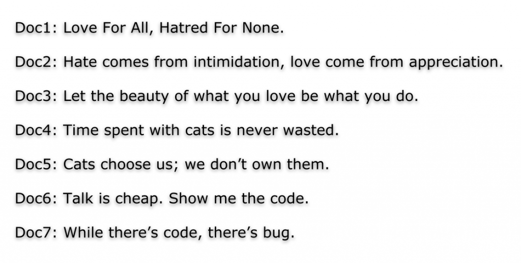
The dataset is composed of documents and it is preferable that these are of various categories so that the groups are as obvious as possible. A very simple dataset that we will use as an example in the following contains only 7 documents, each with a short content.
3. Parsing
There are a number of filters through which a document is passed, and these are:
- Lowercase (ex: “Cat” -> “cat”);
- Remove stopwords (ex: “a,” “and,” “but,” “how,” “or”, “is”, “what” etc.);
- Remove duplicates;
- Keep the words whose part of speech is “NOUN” or “PROPN”;
- Lemmatization.
A vocabulary is created which is composed of the words kept in the documents after processing.
4. TfidfVectorizer
Algorithms have a hard time understanding text data so we need to transform the data into something the model can understand. Computers are exceptionally good at understanding numbers. If we represent the text in each document as a vector of numbers then our algorithm will be able to understand this and proceed accordingly. We will transform the document into a vector of numbers using Term Frequency-Inverse Document Frequency or TF-IDF. The TF-IDF enables to calculate the importance of words in each document relative to what is in that document but also relative to all the documents in the dataset.
def tfidfVectorizer(data, vocabulary):
    tf_idf_vectorizor = TfidfVectorizer(vocabulary=vocabulary)
    tf_idf = tf_idf_vectorizor.fit_transform(data)
    tf_idf_norm = normalize(tf_idf)
    tf_idf_array = tf_idf_norm.toarray()

    return tf_idf_array, tf_idf_vectorizor
| Documents | cat | time | hatred | none | love | code | show | talk | beauty | bug |
|---|---|---|---|---|---|---|---|---|---|---|
| Doc1 | 0.000 | 0.000 | 0.632 | 0.632 | 0.448 | 0.000 | 0.000 | 0.000 | 0.000 | 0.000 |
| Doc2 | 0.000 | 0.000 | 0.000 | 0.000 | 0.448 | 0.000 | 0.000 | 0.000 | 0.000 | 0.000 |
| Doc3 | 0.000 | 0.000 | 0.000 | 0.000 | 0.578 | 0.000 | 0.000 | 0.000 | 0.815 | 0.000 |
| Doc4 | 0.638 | 0.769 | 0.000 | 0.000 | 0.000 | 0.000 | 0.000 | 0.000 | 0.000 | 0.000 |
| Doc5 | 1.000 | 0.000 | 0.000 | 0.000 | 0.000 | 0.000 | 0.000 | 0.000 | 0.000 | 0.000 |
| Doc6 | 0.000 | 0.000 | 0.000 | 0.000 | 0.000 | 0.506 | 0.609 | 0.609 | 0.000 | 0.000 |
| Doc7 | 0.000 | 0.000 | 0.000 | 0.000 | 0.000 | 0.638 | 0.000 | 0.000 | 0.000 | 0.769 |
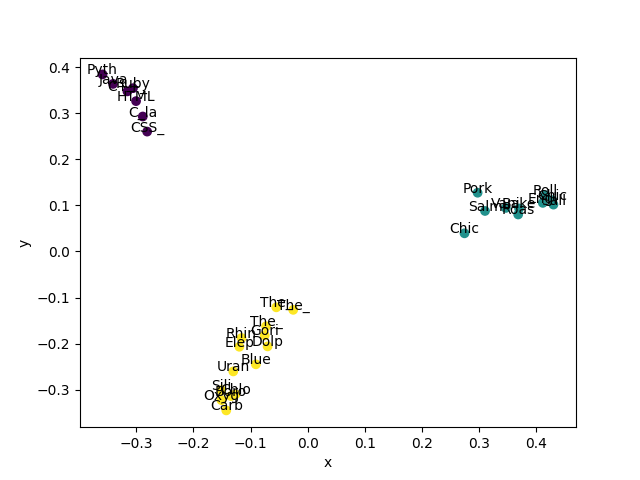
5. PCA
In order to see our clusters graphically, we are going to use Incremental principal component analysis (IPCA) to reduce the dimensionality of our feature matrix so we can plot it in two dimensions. IPCA is typically used as a replacement for principal component analysis (PCA) when the dataset to be decomposed is too large to fit in memory.
def pca(tf_idf_array):
    sklearn_pca = decomposition.IncrementalPCA(n_components=2)
    Y_sklearn = sklearn_pca.fit_transform(tf_idf_array)

    return sklearn_pca, Y_sklearn
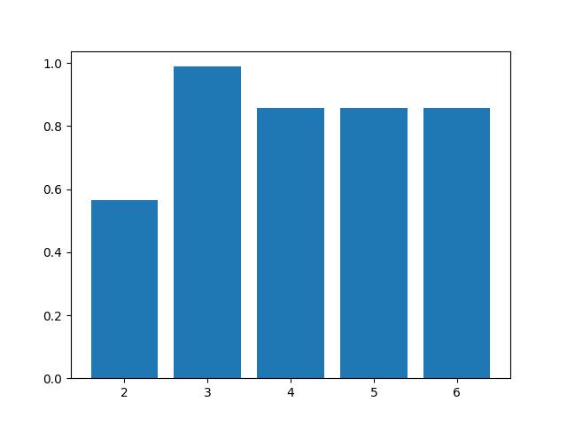
6. The Silhouette Method
When using clustering, one of the things we need to do is make sure we choose the optimal number of clusters. If the number is too little then we could be grouping data together that have significant differences. Also if there are too many clusters then we will just be overfitting the data and our results will not generalise well. We will use the silhouette method which is a common technique used for this task.
Silhouette Score is a measure used to decide the number of clusters to be formulated from the data. It is calculated for each instance and the formula goes like this: Silhouette Coefficient = (x-y) / max(x,y),
where, y is the mean intra cluster distance: mean distance to the other instances in the same cluster. x depicts mean nearest cluster distance i.e. mean distance to the instances of the next closest cluster.
The coefficient varies between -1 and 1. A value close to 1 implies that the instance is close to its cluster is a part of the right cluster. Whereas, a value close to -1 means that the value is assigned to the wrong cluster.
def silhouette_optimal_number_clusters(Y_sklearn, max_clusters=10, iterations=600):
    scores = []
    number_clusters_list = []
    num_clusters_tests = min(len(Y_sklearn), max_clusters)
    for n_clusters in range(2, num_clusters_tests):
    clusterer = Clustering(n_clusters, 1, iterations)
    clusterer.fit(Y_sklearn)
    preds = clusterer.predict(Y_sklearn)
    score = silhouette_score(Y_sklearn, preds)
    scores.append(score)
    number_clusters_list.append(n_clusters)

    max_score = max(scores)
    index = scores.index(max_score)
    optimal_number_clusters = number_clusters_list[index]

    return optimal_number_clusters, scores
The optimal number of clusters for the chosen dataset is 3.
7. Gaussian Mixture Model (GMM)
The classic classification algorithm is K-Means used to cluster data. K-means can handle and find circular clusters because all the distances are defined using Euclidean distance which does not prefer one direction over another. The way that we are going to deal with that is we are going to model our data that is for every cluster we are going to learn a Gaussian distribution that explains what that cluster looks like.
For K-means we had each cluster with a means now we are going to have in addition to a mean we are going to learn a variance. The variance captures properties of the data distribution that we couldn’t with just a mean.
So the Gaussian distribution is defined by a mean and a variance. The mean corresponds to where is the center of the distribution and the variance says how spread out it is.
def cluster(Y_sklearn, optimal_number_clusters):
    test_e = Clustering(optimal_number_clusters, 1, 600)
    test_e.fit(Y_sklearn)
    predicted_values = test_e.predict(Y_sklearn)

    return test_e, predicted_values
8. Feature extraction
What we are mainly interested in is seeing if there are any commonalities between words in each cluster or any particular words that stand out. This is a pretty powerful way of getting a general idea for what the documents contain and can guide any further analysis we wish to do. We can view the top words in each cluster.
def get_top_features_cluster(tf_idf_array, tf_idf_vectorizor, prediction, n_feats):
    labels = np.unique(prediction)
    dfs = {}
    for label in labels:
        id_temp = np.where(prediction == label)
        x_means = np.mean(tf_idf_array[id_temp], axis=0)
        sorted_means = np.argsort(x_means)[::-1][:n_feats]
        features = tf_idf_vectorizor.get_feature_names()
        best_features = [(features[i], x_means[i]) for i in sorted_means]
        dfs[label] = best_features

    return dfs
Below are three tables corresponding to the top 2 words in each cluster ordered by relative importance as measured by TF-IDF.
Cluster 1
Documents: Doc1.md, Doc2.md, Doc3.md
| Feature | Score |
|---|---|
| love | 0.4918478905261349 |
| beauty | 0.2718546425106399 |
Cluster 2
Documents: Doc4.md, Doc5.md
| Feature | Score |
|---|---|
| cat | 0.8193542741781095 |
| time | 0.38472437869749426 |
Cluster 3
Documents: Doc6.md, Doc7.md
| Feature | Score |
|---|---|
| code | 0.5724554669787523 |
| bug | 0.38472437869749426 |

Written by
Sara
Sara is a Machine Learning / Fullstack Engineer, part of the AscentCore Research Lab team